So deep learning has taken the world by storm. Frameworks for training deep neural networks, like TensorFlow, allow you to construct so-called differentiable programs. The idea is that one can compute the derivative of some program (usually some neural net), and then use that to optimize its parameters.

I wrote this post to introduce researchers in the verification and programming languages community to automatic differentiation of programs. The assumption is that—extrapolating from myself here—you got into this field for the love of logic and discrete math (and an unhealthy aversion to continuous mathematics).

Programming language

Let’s consider a very simple programming language where there are no loops or conditions, just a sequence of assignment statements of the form:

Here, $c$ is a real-valued constant and $v_i$ are real-valued program variables. Any program $P$ in this language is assumed to have a single special input variable $x$ and an output variable $y$.

$P$ is also assumed to be in static single assignment (SSA) form—i.e., each variable gets assigned to at most once. This is equivalent to continuation-passing style (CPS). If you’ve used TensorFlow, the computation graph that you construct there is effectively a program in SSA, where each graph node represents one variable’s assignment.

Example program

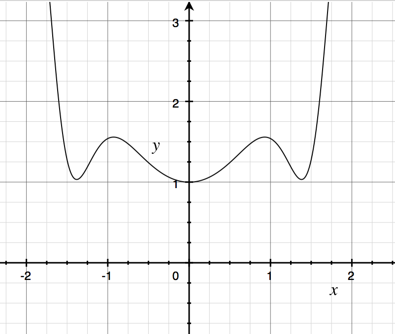
Note that programs in our language are functions in $\mathbb{R} \to \mathbb{R}$. Consider the function $f(x) = x^2 + cos(x^2)$. We can write this in our language as the program $P$ below:

If you plot this function, you get the following spooky graph:

If you remember your calculus, the partial derivative of a function $\frac{\partial f}{\partial x}$ is essentially the rate of change of the output $y$ as $x$ changes. For our function $f$,

Notice that $\frac{\partial f}{\partial x}(0) = 0$, since $x = 0$ is a stationary point, so the rate of change at that point is 0.

Technically, we’re computing total derivatives in this post, since we only have one input variable $x$, which I enforce for simplicity. The general methodology I lay out here easily extends to functions with multiple input arguments.

Language semantics

The semantics of our little language is standard. A state $s$ of a program $P$ is a map from variables to real numbers. The function $\textit{post}$ below takes a program and a state $s$ and returns the state resulting from executing $P$:

1. $\textit{post}(P_1;P_2, s) \triangleq \textit{post}(P_2,\textit{post}(P_1,s))$
2. $\textit{post}(v_1 \gets c, s) \triangleq s[v_1 \mapsto c]$
3. $\textit{post}(v_1 \gets v_2 \times v_3, s) \triangleq s[v_1 \mapsto s(v_2) \times s(v_3)]$
4. $\textit{post}(v_1 \gets v_2 + v_3, s) \triangleq s[v_1 \mapsto s(v_2) + s(v_3)]$
5. $\textit{post}(v_1 \gets cos(v_2), s) \triangleq s[v_1 \mapsto cos(s(v_2))]$

Above, $P_1;P_2$ denotes sequential composition, $s(v)$ denotes the value of $v$ in state $s$, and $s[v \mapsto c]$ denotes state $s$ but with $v$ mapping to the value $c$.

Forward differentiation

We will now extend the semantics such that evaluating $P$ on input $x$ not only returns $P(x)$, but also $\frac{\partial P}{\partial x}(x)$, the partial derivative of $P$ w.r.t. the input variable $x$.

Below, we define the new semantics with a function $\partial\textit{post}$, where we keep track of two copies of the program variables, the variables $v_i$ and a new copy $\dot v_i$, which denotes the rate of change of $v_i$ w.r.t. the input $x$, i.e.,

Finally, when the program terminates with the new semantics, we can recover the variable $\dot y$, which will hold the value $\frac{\partial P}{\partial x}(x)$.

Note that, by definition, $\dot x = 1$.

Sequential composition

For sequential composition, $P_1;P_2$, $\partial\textit{post}$ behaves just like $\textit{post}$.

Constant assignment

For the constant assignment $v_1 \gets c$, we have

In other words, the rate of change of $v_1$ is zero, since it’s not dependent on $x$ in any way.

Addition

For addition, we have

That is, the rate of change of $v_1$ is the sum of the rates of change of $v_2$ and $v_3$.

Multiplication

For multiplication,

In other words, the rate of change of $v_1$ w.r.t. $x$ is the rate of change of $v_2$, scaled by $v_3$, plus the rate of change of $v_3$, scaled by $v_2$.

Trigonometric functions

For cosine, we have

This follows from the chain rule, which says that the rate of change of $f(u)$ is the rate of change of $f$ scaled by the rate of change of its argument $u$. You might remember that the derivative of $cos(x)$ is $-sin(x)$, so, following the chain rule, we simply scale $-sin(v_2)$ by $\dot v_2$.

Example continued

Continuing our above example with the program $P$ encoding the function $f(x) = x^2 + cos(x^2)$, we can now execute $P$ using our new semantics. Say, we begin executing $P$ from the state where $x = 0$. At the end of the execution, we will get a state where $y = 1$, and $\dot y = 0$.

Let’s step through the program one instruction at a time, maintaining both copies of the variables at every point along the way.

Notes

I covered the simpler case of forward differentiation, which proceeds by executing the program in a forward manner. For functions with more than one input, it is more efficient to perform backward differentiation, which the popular backpropagation algorithm is an instance of. Adapting the above semantics to backpropagation is not hard, it’s just messier, as we have to execute the program forward and then backward. Therefore, I decided to illustrate the forward mode only. For more information, I encourage you to read the excellent survey by Baydin et al., which heavily influenced my presentation.

Thanks to Kartik Agaram, Ben Liblit, and David Cabana for catching typos and errors.