A Quantum Circuit Simulator in 27 Lines of Python
Aws Albarghouthi
We’re going to write a quantum circuit interpreter (or simulator) using just 27 lines of Python!
To understand this post, you don’t need to know anything about quantum computing. All you need to know is matrix multiplication! I’ll walk you through the rest! We’re going to treat the operations of a quantum computer as yet another programming language for which we want to build an interpreter. So we won’t get too much into quantum mechanics or fancy quantum algorithms.
You can find the entire simulator code at the bottom of this post, or as a notebook.
Classical circuits
We will begin by writing an interpreter for classical circuits—you know, good old not, and, or. Then, we will generalize our interpreter to quantum circuits. A classical circuit in our setting applies logical operations to $n$ bits.
Classical state
Let’s begin by representing the state of $n$ bits. We’ll do this in an unusual way. We will define a Boolean vector (i.e., a vector of 0s and 1s) of size $2^n$ where each index of the vector represents one possible state of the $n$ bits. There will be a single non-zero (1) element in the vector indicating the state.
For $n=1$, we have a vector of size 2, e.g.:
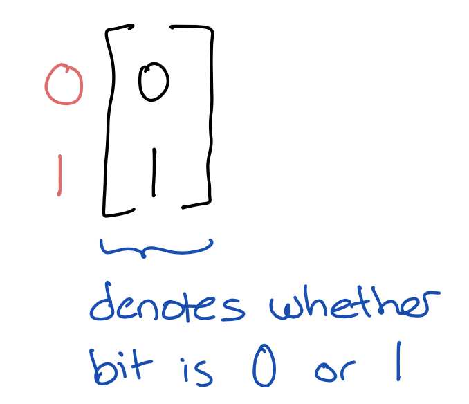
The vector is in black; the numbers in pink (left) are the indices denoting the state of the bit. The vector above, therefore, represents a bit that is set to 1, since it has element 1 at index 1. Similarly, the vector \(\begin{bmatrix} 1\\0 \end{bmatrix}\) denotes a bit set to 0, because it has element 1 at index 0.
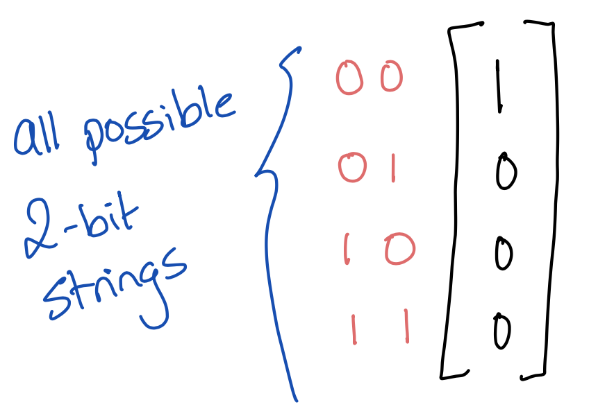
For $n=2$, we have a vector of size 4, like the following, which denotes that both bits are 0, because it has element 1 at index 00.
You get the idea. It’s a terribly inefficient representation, but I chose it on purpose because we’ll later generalize it to qubits, and quantum simulation is inherently inefficient as far as we can tell.
Here’s a Python class to represent a classical state with $n$ bits.
Note that a state is initialized to all bits being 0.
Also, note that we’re using numpy (np)
class Cstate:
  def __init__(self, n):
    # number of bits
    self.n = n

    # create vector of size 2^n
    self.state = np.zeros(2**self.n, dtype=int)

    # initialize bits to 0s
    # by setting index 0 of vector to 1
    self.state[0] = 1
For example, the state field for 2 bits initially looks like this,
denoting the state 00 (just like the 2-bit vector illustrated above)
[1 0 0 0]
Numpy represents vectors as rows instead of columns like we do—it won’t make a difference for us.
Flipping a bit
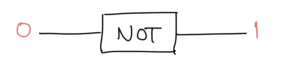
Let’s now apply a NOT (negation) operation to a bit. In a circuit of 1 bit, this looks as follows (where the pink stuff is an example input/output of the circuit):
NOT is a transformation that takes a bit from one state to another. We’re going to represent it as a transformation matrix:
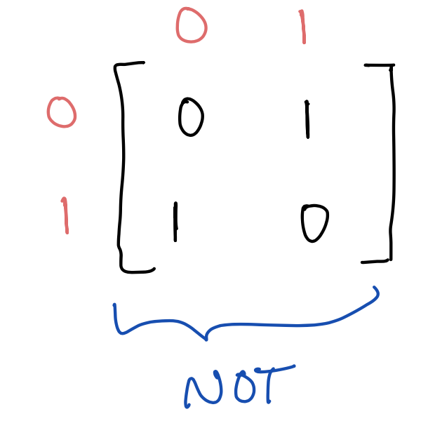
The way to read the matrix is by looking at columns then rows. Note that each column has a single 1 and the rest of the entries are 0. The position of the 1 denotes the transformation. Take the bottom left 1 in the matrix, which is at column 0 and row 1; this means that a bit that is 0 is transformed into 1. Take the top right 1 now, at column 1 and row 0; this means that a bit that is 1 is transformed into 0.
Now to apply this transformation to a state in our representation, we simply multiply the NOT matrix above with the state vector. For example, we can apply NOT to a single bit set to 0:
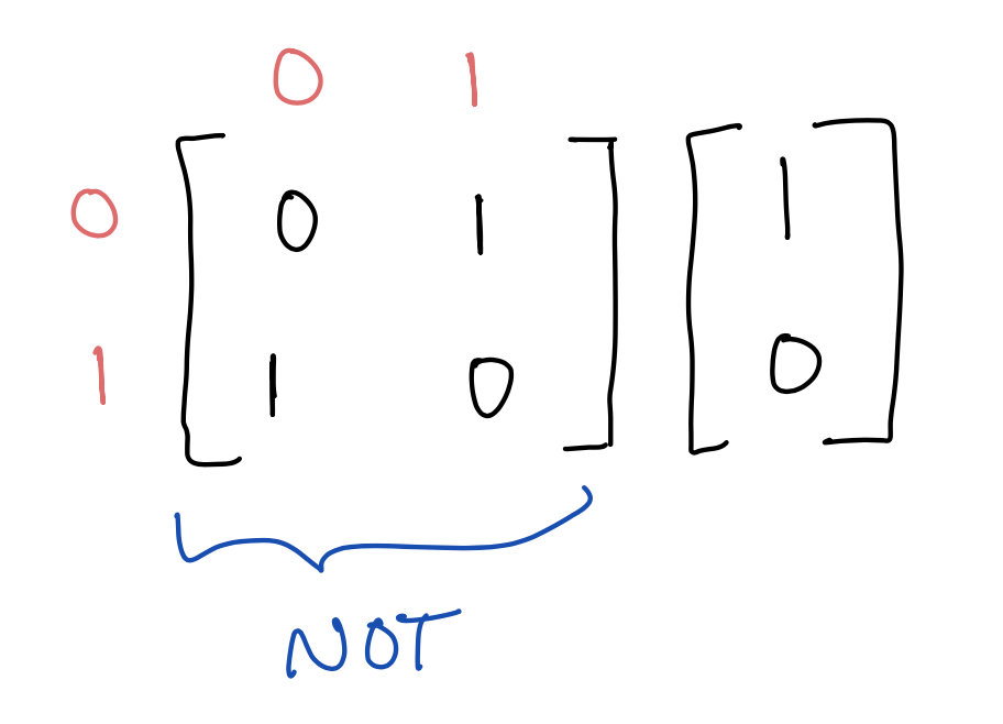
The above multiplication results in \(\begin{bmatrix} 0\\1 \end{bmatrix}\), denoting a bit set to 1.
Intuitively, multiplication by a transformation matrix simply moves around the 1 in the input state vector to some other position in the output state vector.
Handling multiple bits
But what happens when we have $n$ bits and we only want to negate a specific one, say the $i$th one?
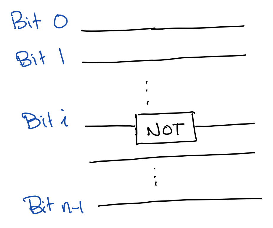
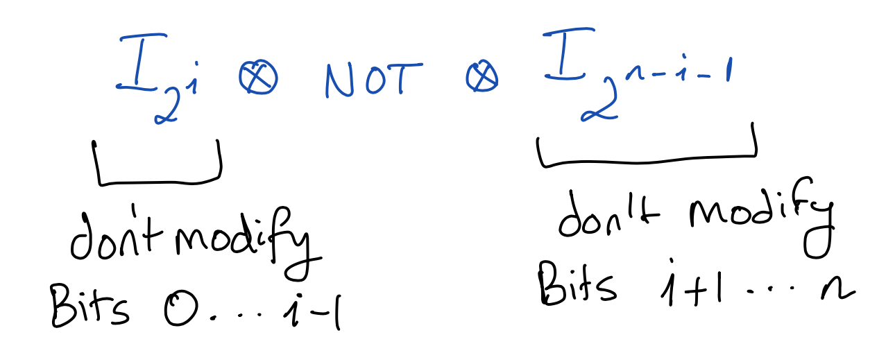
We will construct a bigger transformation matrix that only applies the NOT to the $i$th bit and leaves the rest untouched. To do so, we will “compose” the NOT matrix with two identity matrices. One identity matrix will say that all bits before bit $i$ (bits $0$ to $i-1$) are untouched; the other will say that all bits after bit $i$ (bits $i+1$ to $n-1$) are untouched.
Let’s first do this for the simple case of two bits where we want to negate the second bit. We take the Kronecker product ($\otimes$) of the identity matrix (of size 2, denoted $I_2$) with the NOT transformation.
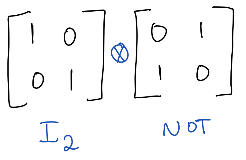
If you haven’t seen Kroenecker product before, don’t be scared; it just multiplies each element of the left matrix with the entire right matrix. So in this case, we get a $4 \times 4$ matrix as follows:
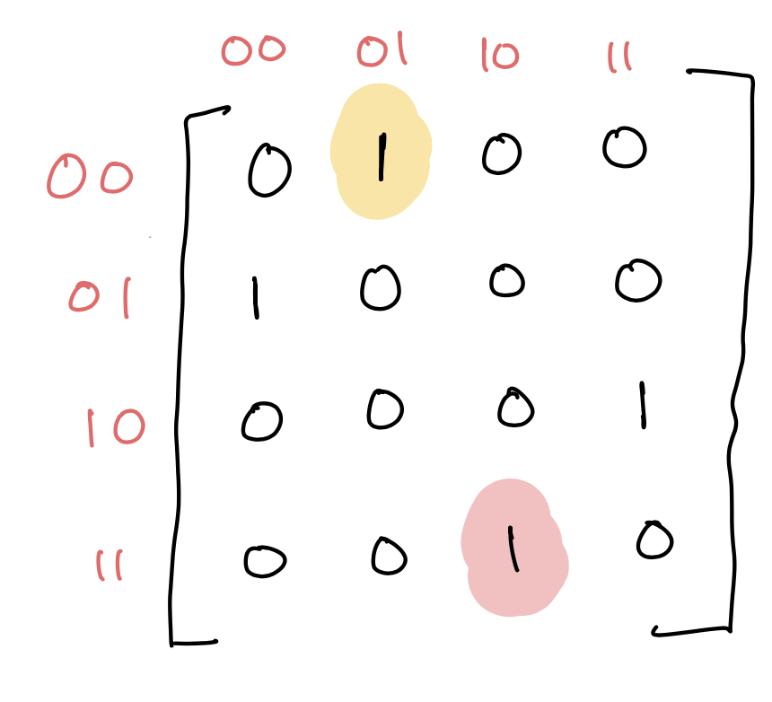 Look at the $2 \times 2$ sub-matrix on the top left.
It’s the result of multiplying 1 (the top-left element of $I_2$) with the NOT matrix.
Look at the $2 \times 2$ sub-matrix on the top left.
It’s the result of multiplying 1 (the top-left element of $I_2$) with the NOT matrix.
Consider the element highlighted in yellow. It says that if the bits are 01 (column), then turn them into 00 (row). Observe that the second bit flips, but not the first bit, as desired. The same can be seen with the element highlighted in pink.
Alright, let’s capture this Kronecker product idea in its general form and implement it. $I_m$ is an indentity matrix that of size $m \times m$.
We will implement this as a method of the Cstate class
that takes an arbitrary transformation matrix t over contiguous bits and
applies it to all $n$ bits.
eye is numpy’s identity matrix function,
kron is Kronecker product,
and matmul is matrix multiplication.
def op(self, t, i):
    # I_{2^i}
    eyeL = np.eye(2**i, dtype=int)

    # I_{2^{n-i-1}}
    # log2(t.shape[0]) denotes how many bits t applies to
    # in case of NOT, log2(t.shape[0]) == 1
    eyeR = np.eye(2**(self.n - i - int(np.log2(t.shape[0]))),
        dtype = int)

    # eyeL ⊗ t ⊗ eyeR
    t_all = np.kron(np.kron(eyeL, t), eyeR)

    # apply transformation to state
    self.state = np.matmul(t_all, self.state)

def NOT(self, i):
    not_matrix = np.array([
        [0,1],
        [1,0]
    ])
    self.op(not_matrix, i)
The method op takes a transformation matrix t, e.g., the NOT matrix,
and applies it to the bit i.
The NOT method calls op with the NOT matrix.
Note that op also works with operations that apply to more than 1 bit,
e.g., AND, so long as the bits are contiguous.
Binary operations
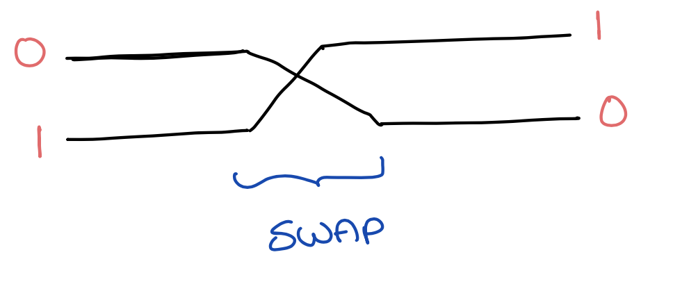
Let’s now look at some binary operations. The following transformation swaps two bits.
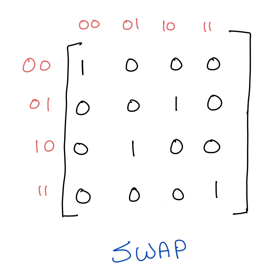
We can implement it as follows.
Note that swap(i) swaps bits i and i+1.
def swap(self, i):
    swap_matrix = np.array([
        [1, 0, 0, 0],
        [0, 0, 1, 0],
        [0, 1, 0, 0],
        [0, 0, 0, 1]
    ])
    self.op(swap_matrix, i)
As a circuit, a swap is shown like this:
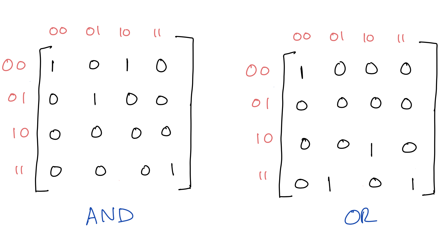
We can similarly implement AND and OR, where the result is stored
in the first of the two bits.
Simple example
Finally, we end our discussion of classical circuits with a simple circuit that checks if two bits are both zero. The result is stored in the first bit.
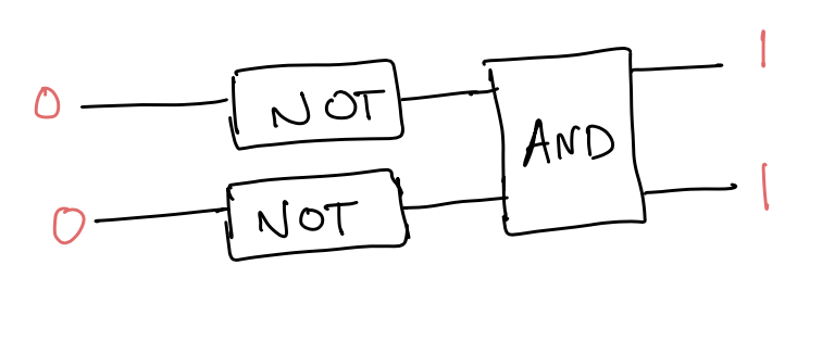
# initialize state
# Recall that Cstate initializes all bits to 0
s = Cstate(2)
s.NOT(0) # negate first bit
s.NOT(1) # negate second bit
s.AND(0) # AND first and second bits

print(s.state)
We get
[0 0 0 1]
which means that the final state of the 2 bits is 11. Since the first bit is 1, this means that the two bits were initially zero.
In summary, with AND, OR, and NOT we can write an arbitrary Boolean function from $n$ bits to $n$-bits as a sequence of Cstate operations. Each one of these Cstate operations is implemented using matrix multiplication,
and the state of the bits is encoded as a vector of size $2^n$
with a single 1 denoting the state.
Quantum circuits
We now generalize the above to quantum circuits. Instead of bits, we have qubits. A qubit can be 0, 1, or a superposition of 0 and 1. So if you write out its vector, it can have numbers in different indices. E.g.,
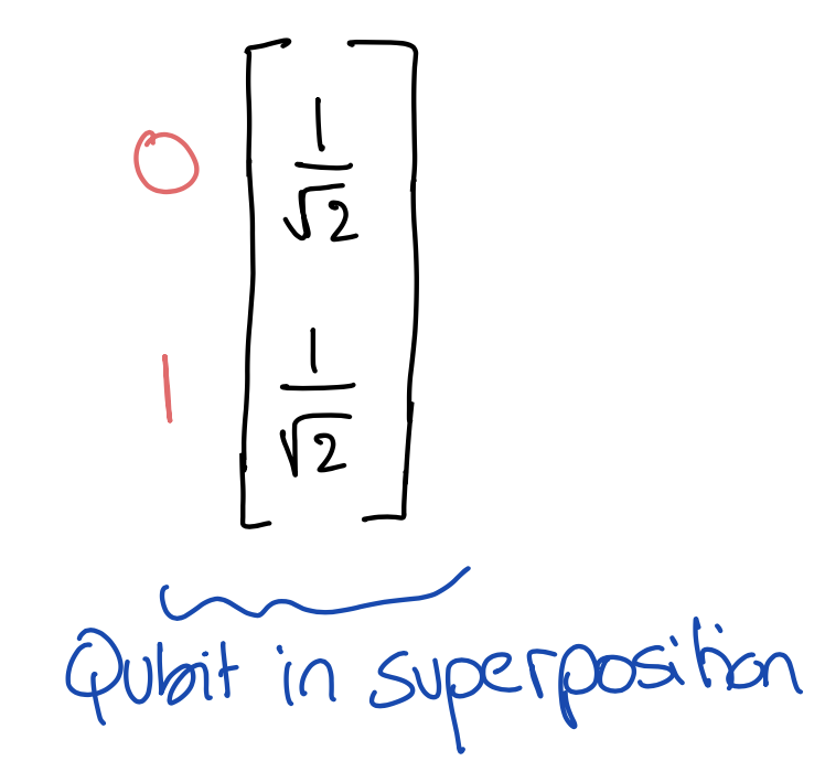
What this says is that if you measure the qubit—read its value—you will read 0 with probability 1/2 and 1 with probability 1/2. The probability is the sqaure of the absolute value of $1/\sqrt{2}$, the amplitude. Amplitudes can be complex numbers. If you sum up the squares of absolute amplitudes, you should get 1, since they encode a probability distribution. In the above example, we have
\[\left\vert\frac{1}{\sqrt{2}}\right\vert^2 + \left\vert\frac{1}{\sqrt{2}}\right\vert^2 = 1\]The above qubit vector is usually written with the following notation: \(\frac{1}{\sqrt{2}} \vert0\rangle + \frac{1}{\sqrt{2}} \vert1\rangle\). Amplitudes are multiplied by the classical states, 0 and 1, which are wrapped in the notation \(\vert\cdot\rangle\) for historical reasons.
We can easily represent this quantum state by copy-pasting the class definition
of classical states and changing the types from int to complex.
Who said copy-paste is bad?
Voila! We now have a quantum state class Qstate.
class Qstate:
  def __init__(self, n):
    self.n = n
    self.state = np.zeros(2**self.n, dtype=complex)
    self.state[0] = 1 #initialize qubits to 0s
Hadamard gate
Transformations of quantum states are also matrices, but they can have complex numbers. The matrices are unitary, which means that they are invertible and maintain that the state represents a probability distribution. This fact comes from the postulates of quantum mechanics, but doesn’t really concern us when implementing an interpreter. It’s interesting to note though that AND and OR are not unitary, because they’re not reversible, and therefore are not quantum operations.
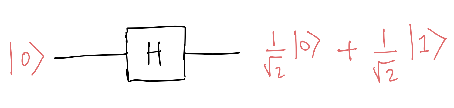
The first transformation we’ll look at is Hadamard, which applies to a single qubit.
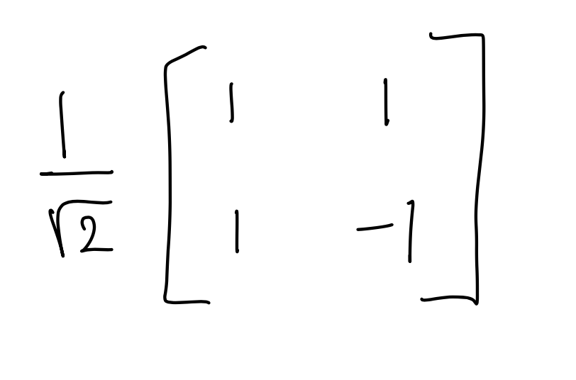
A Hadamard gate puts a state in superposition. For example, given the classical state $\vert0\rangle$, i.e., the vector \(\begin{bmatrix} 1\\ 0 \end{bmatrix}\), it transforms it into the superposition we saw above,
\[\frac{1}{\sqrt{2}} \vert0\rangle + \frac{1}{\sqrt{2}} \vert1\rangle\]As a circuit, we write this as follows:
Similarly, given the state $\vert1\rangle$, Hadamard transforms it into the superposition
\[\frac{1}{\sqrt{2}} \vert0\rangle - \frac{1}{\sqrt{2}} \vert1\rangle\]or equivalently the vector
\[\begin{bmatrix} \frac{1}{\sqrt{2}} \\ - \frac{1}{\sqrt{2}} \end{bmatrix}\]Note the negative amplitude of $\vert1\rangle$. This is a key property of quantum mechanics that quantum algorithms exploit, allowing amplitudes to cancel out (interfere), which we cannot achieve with classical randomized algorithms. We won’t get into it, but I recommend taking a look at Grover’s algorithm (which is beautiful).
We will implement Hadamard just as we did with NOT.
I’m using isq2 as a shorthand for $1/\sqrt{2}$.
# this function is the same as in the classical case
# the only difference is dtype, which is complex now
def op(self, t, i):
    #I_{2^i}
    eyeL = np.eye(2**i, dtype=complex)

    #I_{2^{n-i-1}}
    eyeR = np.eye(2**(self.n - i - int(np.log2(t.shape[0]))),
        dtype = complex)

    # eyeL ⊗ t ⊗ eyeR
    t_all = np.kron(np.kron(eyeL, t), eyeR)

    # apply transformation to state
    self.state = np.matmul(t_all, self.state)

def hadamard(self, i):
    h_matrix = isq2 * np.array([
      [1,1],
      [1,-1]
    ])
    self.op(h_matrix, i)
Controlled NOT gate
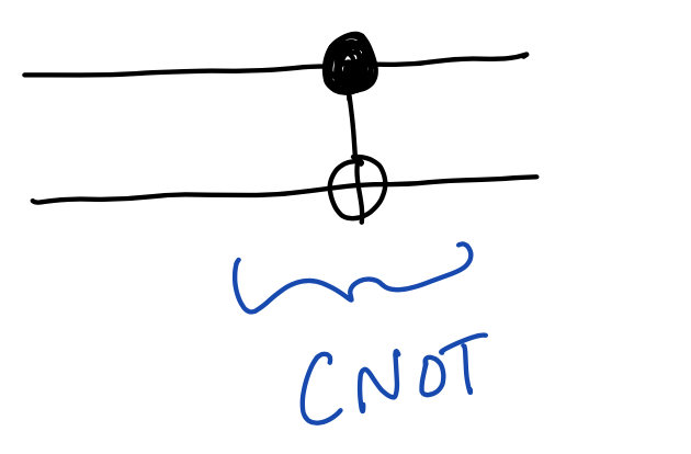
Next, we’ll look at the CNOT (controlled NOT) gate, which is a binary gate.
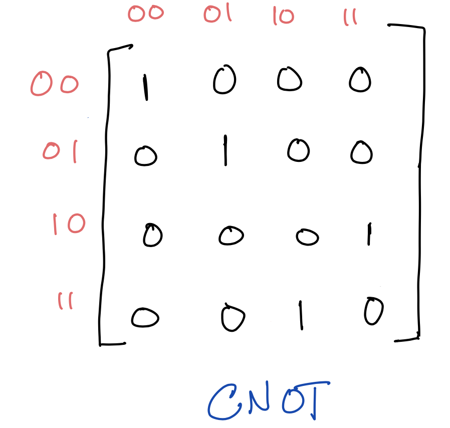
Classically speaking, this takes the XOR of two bits and stores the result in the second bit. But, as we shall see, it is fundamental in quantum computing, as it allows us to entangle two qubits (more on this in a bit). Pictorially, CNOT is denoted as follows:
Again, we will implement CNOT just like in the classical setting:
def cnot(self, i):
  cnot_matrix = np.array([
      [1, 0, 0, 0],
      [0, 1, 0, 0],
      [0, 0, 0, 1],
      [0, 0, 1, 0]
  ])
  self.op(cnot_matrix, i)
Qubit swaps are the same as classical bit swaps.
Phase-shift gates
In the classical setting, AND and NOT suffice to implement any Boolean function. In the quantum setting, we’re missing two single-bit gates that give us the full power of a quantum computer. By full power, I mean a set of gates that can approximate any unitary transformation to an arbitrary degree of accuracy.
The two missing gates are the $S$ and $T$ gates. These gates don’t change the probability of measurement, but they change the phase of the amplitudes. This is where complex numbers come into play.
We’ll take a look at the $S$ gate:
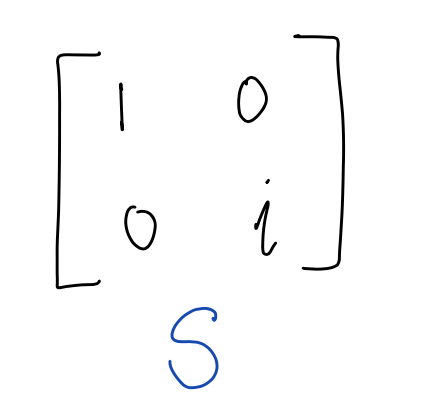 Applying $S$ to a state doesn’t change the amplitude of $\vert0\rangle$,
but it multiplies the amplitude of $\vert1\rangle$ by $i$—the imaginary unit. (Remember complex numbers?)
For example, if we apply $S$ to the superposition state, we get:
Applying $S$ to a state doesn’t change the amplitude of $\vert0\rangle$,
but it multiplies the amplitude of $\vert1\rangle$ by $i$—the imaginary unit. (Remember complex numbers?)
For example, if we apply $S$ to the superposition state, we get:
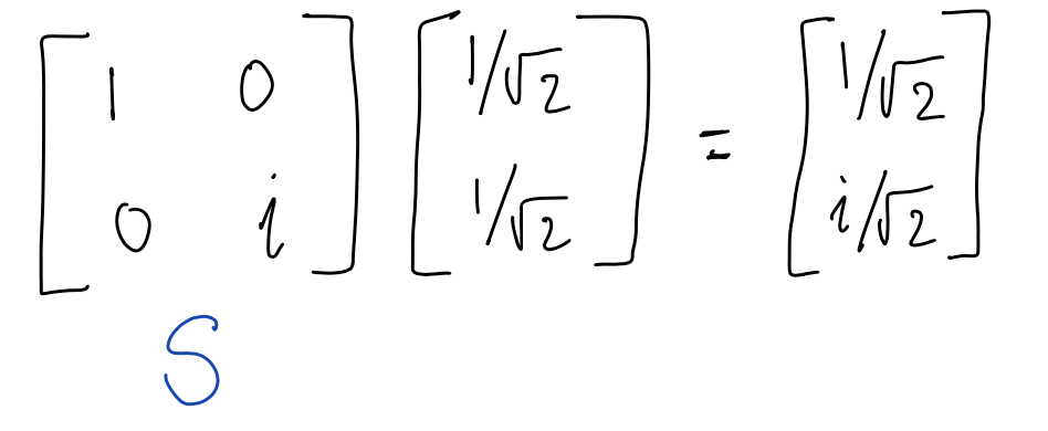 Check out how the amplitude of $\vert1\rangle$
changed to $i / \sqrt{2}$.
If we turn the amplitude of $\vert 1 \rangle$ into a probability, we get the same probability as before:
Check out how the amplitude of $\vert1\rangle$
changed to $i / \sqrt{2}$.
If we turn the amplitude of $\vert 1 \rangle$ into a probability, we get the same probability as before:
So while the amplitude has changed, the probabilities haven’t.
Here are the $S$ and $T$ gates in code. Note that numpy uses $j$ instead of $i$ for the imaginary unit. The $T$ gate is similar to the $S$ gate, in that it only changes the amplitude of $\vert1\rangle$, but it changes it in a different way.
# S gate
def s(self, i):
  s_matrix = np.array([
      [1,0],
      [0,1j]
  ])
  self.op(s_matrix,i)

# T gate
def t(self, i):
  t_matrix = np.array([
      [1,0],
      [0,isq2 + isq2 * 1j]
  ])
  self.op(t_matrix, i)
EPR pairs
At this point, we have a full-blown quantum-circuit simulator. You can always add more gates as needed, but we have already implemented a universal gate set.
We will end with constructing an EPR pair, a special entangled state of two qubits proposed by Einstein, Podolsky and Rosen in 1935 to argue that quantum mechanics is incomplete.
Here’s how the circuit looks. Apply a Hadamard to the first qubit,
putting it in superposition, then apply a CNOT to both qubits.
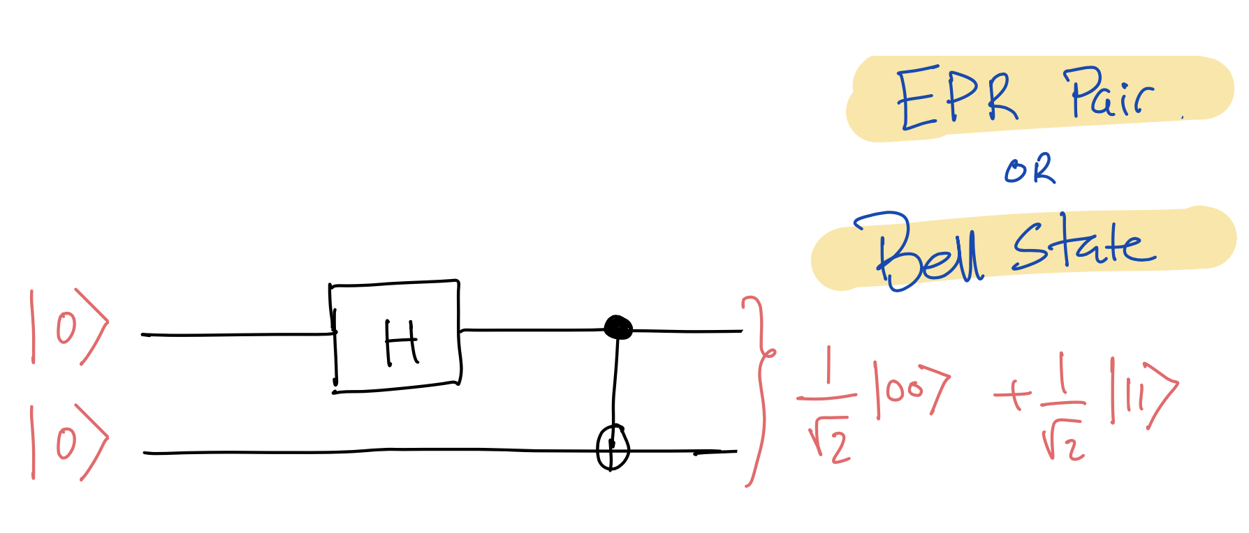
This results in the following state, which is called an EPR pair or a Bell state:
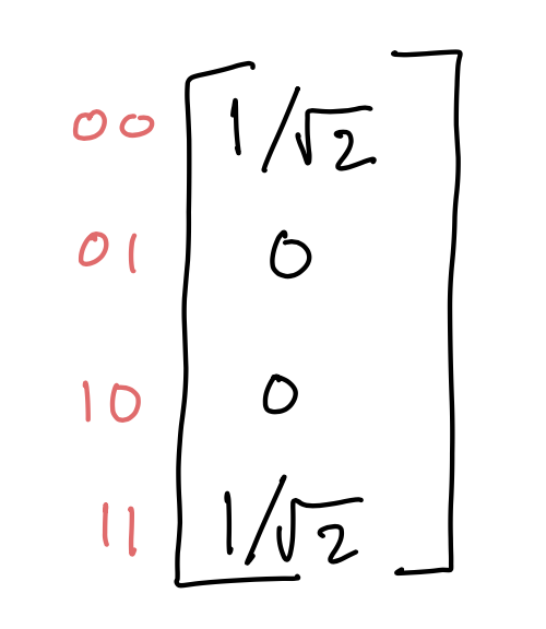
\[\frac{1}{\sqrt{2}} \vert00\rangle + \frac{1}{\sqrt{2}} \vert11\rangle\]In vector notation, an EPR pair is
The beauty of this state is that the two qubits are entangled. This means that if we measure the first bit, we will get 0 or 1 with equal probability. But then the other qubit will also collapse to the same answer that we get. So if each of us has one of the two entangled bits, it appears that we can achieve instantaneous communication! This didn’t sit well with Einstein and his friends. Indeed, their construction of EPR pairs was to demonstrate a paradox. EPR pairs are key ingredients in quantum teleportation, which I encourage you to read about.
Here’s how we construct an EPR pair with our interpreter.
# constructing an EPR pair
s = Qstate(2) # create a 2-qubit state
s.hadamard(0) # hadamard on first qubit
s.cnot(0) # CNOT the two qubits

print(s.state)
We get the following output, which I’ve simplified for legibility. (Note that $1/\sqrt{2} \approx 0.70710678$)
[0.70710678 0 0 0.70710678]
Notes
That’s it, folks. We’ve implemented a quantum circuit simulator.
- Our simulator will get exponentially slower with more qubits. This is sadly unavoidable. Nonetheless, researchers have come up with lots of techniques to make quantum simulations faster on classical computers, e.g., using BDDs and parallelism.
- Our simulator doesn’t implement measurement, because it represents the entire probability distribution explicitly.
- Our binary gates apply to contiguous (qu)bits.
This makes the
opfunction simpler to write. We can generalize theopfunction to apply binary gates to any pair of (qu)bits, but it gets uglier. Since we haveswap, we can always move qubits next to each other. - As an introduction to quantum computing, I recommend Matuschak and Nielsen’s Quantum Country.
Thanks to John Cyphert for his insightful comments.
The Entire Quantum Circuit Simulator
Here are all 27 lines of code.
import numpy as np

isq2 = 1.0/(2.0**0.5)

class Qstate:
  def __init__(self, n):
    self.n = n
    self.state = np.zeros(2**self.n, dtype=complex)
    self.state[0] = 1

  # apply transformation t to bit i
  # (or i and i+1 in case of binary gates)
  def op(self, t, i):
    # I_{2^i}
    eyeL = np.eye(2**i, dtype=complex)

    # I_{2^{n-i-1}}
    # log2(t.shape[0]) denotes how many bits t applies to
    # in case of NOT, log2(t.shape[0]) == 1
    eyeR = np.eye(2**(self.n - i - int(np.log2(t.shape[0]))),
        dtype = complex)

    # eyeL ⊗ t ⊗ eyeR
    t_all = np.kron(np.kron(eyeL, t), eyeR)

    # apply transformation to state (multiplication)
    self.state = np.matmul(t_all, self.state)

  # Hadamard gate
  def hadamard(self, i):
    h_matrix = isq2 * np.array([
        [1,1],
        [1,-1]
    ])
    self.op(h_matrix, i)

  # T gate
  def t(self, i):
    t_matrix = np.array([
        [1,0],
        [0,isq2 + isq2 * 1j]
    ])
    self.op(t_matrix, i)

  # S gate
  def s(self, i):
    s_matrix = np.array([
        [1,0],
        [0,0+1j]
    ])
    self.op(s_matrix,i)

  # CNOT gate
  def cnot(self, i):
    cnot_matrix = np.array([
        [1, 0, 0, 0],
        [0, 1, 0, 0],
        [0, 0, 0, 1],
        [0, 0, 1, 0]
    ])
    self.op(cnot_matrix, i)

  # Swap two qubits
  def swap(self, i):
    swap_matrix = np.array([
        [1, 0, 0, 0],
        [0, 0, 1, 0],
        [0, 1, 0, 0],
        [0, 0, 0, 1]
    ])
    self.op(swap_matrix, i)